Photogrammetry is the art and science of reconstructing 3D geometry from 2D images. In this post, I’ll walk you through the full pipeline, from a simple set of photos to a detailed 3D mesh.
Pipeline Overview:
- Input Images: Overlapping photos of a scene or object
- Feature Extraction & Matching: Detect and match keypoints between views
- Sparse Reconstruction: Estimate camera poses and triangulate a sparse 3D point cloud using Structure-from-Motion
- Dense Reconstruction: Build a high-resolution point cloud using multi-view stereo
- Normals Estimation: Compute surface normals from the dense cloud
- Mesh Generation: Construct the final 3D mesh
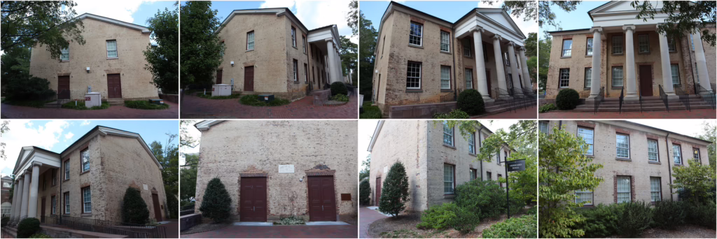
Input Images
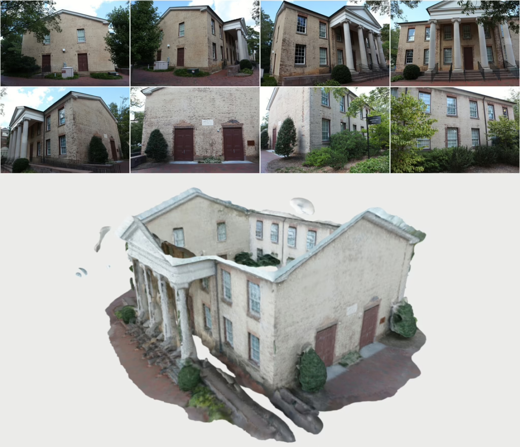
To start, you need multiple images of your subject taken from different viewpoints. It’s important to move around the object rather than just rotating the camera. Translation is key for recovering depth information. Simply rotating the camera will only produce a panorama, not a 3D model. Also, ensure there’s significant overlap between images so the software can find enough matching features. For this example, I used the Gerrard Hall dataset from COLMAP, which contains 100 images of a building taken with the same camera. They look like this:
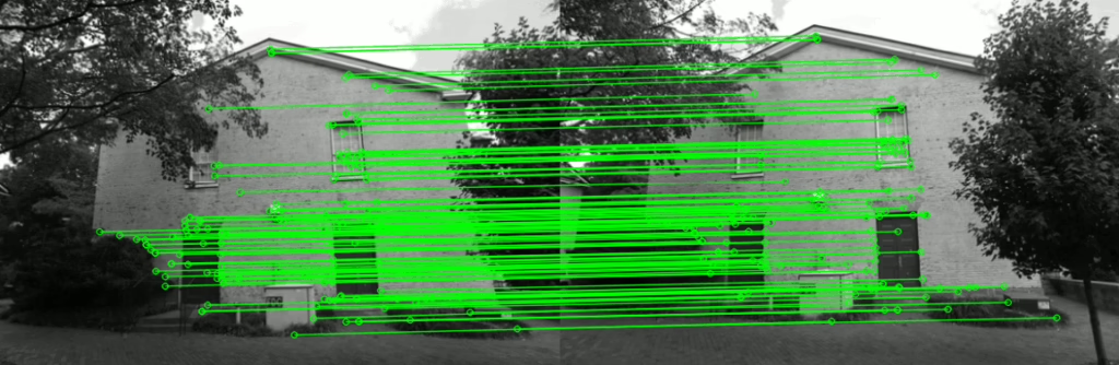
Feature Extraction & Matching
To align images, we first extract keypoints (distinctive features in each photo) using algorithms like SIFT. Then, we match these features between image pairs using a matcher such as FLANN. To reduce false matches, we apply Lowe’s ratio test, which keeps only the matches where the closest descriptor is significantly better than the second-best (typically with a ratio threshold of 0.75). Next, we apply RANSAC to estimate a homography and identify consistent matches, called inliers, based on geometric alignment. This combined filtering ensures that only accurate, reliable matches are used for 3D reconstruction.
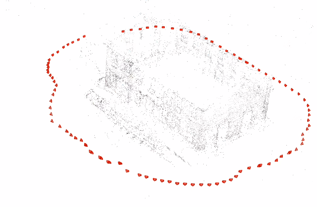
Sparse Reconstruction
Once features are matched, we estimate the camera poses using Structure-from-Motion (SfM). This process incrementally recovers the position and orientation of each camera. With these poses and the matched features, we triangulate 3D points to build a sparse point cloud, which is a rough representation of the scene’s geometry.
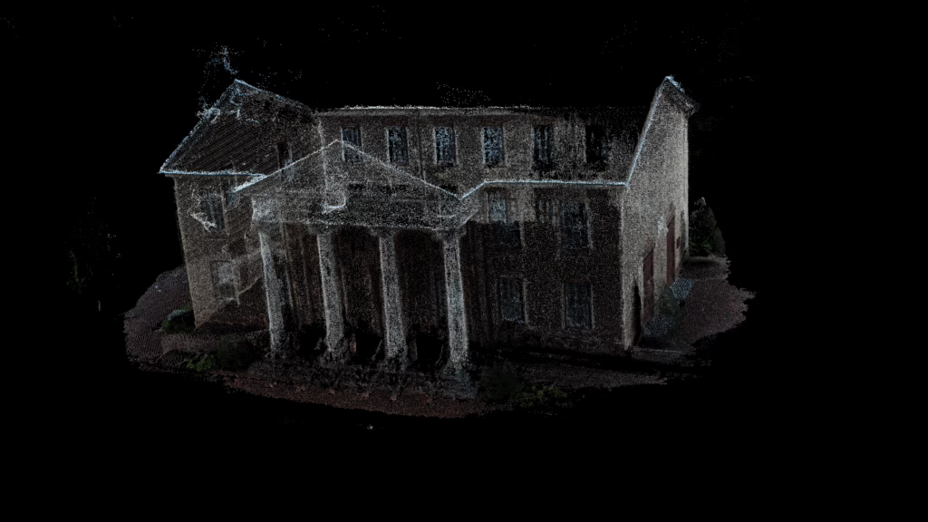
Dense Reconstruction
Sparse reconstruction gives us a structural backbone, but to capture finer detail, we need dense data. Using techniques like multi-view stereo (MVS) or depth map fusion, we generate a dense point cloud by estimating depth for many or all image pixels. This dense representation reveals intricate surface features and prepares the data for meshing.
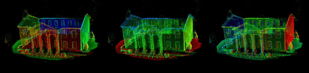
Normals Estimation
With a dense point cloud available, we can estimate surface normals, which are vectors that indicate the direction each surface is facing. Normals are typically computed by analysing a point’s local neighborhood using methods like PCA, or derived directly from mesh geometry. They are essential for realistic rendering, lighting, and further geometric processing.
Mesh Generation
From the dense point cloud and normals, we create a continuous 3D surface. Algorithms such as Poisson surface reconstruction, Delaunay triangulation, or ball-pivoting connect nearby points into a mesh of triangles. The resulting 3D mesh accurately models the object’s shape and can be used in a variety of applications including visualisation, simulation, 3D printing, and CAD.
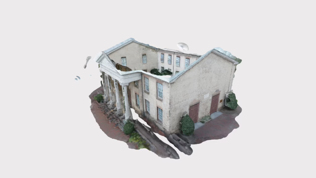
At this point, you have a full 3D mesh reconstructed from your photos. You can now refine it further by cleaning up noise, filling holes, simplifying the mesh, or even texturing it using the original images. The final model can be exported for rendering, editing, or integration into other workflows.
And that’s it! Starting from a simple photo set, you can produce a complete and accurate 3D model of a real-world object or scene.